
Mega-Caps Earn Real Alpha, and Your Models Miss It
Introducing Research-grounded Investor Q&A. Have an interesting idea and would like a thesis check grounded on academic research? Email your query to kp@academicsignal.com and our Research Fellows will tackle the most interesting questions.
In this week’s report:
Mega-caps earn alpha because their idiosyncratic risk can't be diversified away
Your alpha estimates are probably wrong
Research-grounded Investor Q&A: “Does unusual options activity (put-call ratio + volume spikes) predict post-earnings announcement drift direction?” [Premium Content]
1. Mega-caps earn alpha because their idiosyncratic risk can't be diversified away
Idiosyncratic Risk Premium (December 12, 2025) - Link to paper
TLDR
Traditional theory says idiosyncratic (company-specific) risk shouldn't earn alpha because investors can diversify it away
But when the market is highly concentrated, mega-cap idiosyncratic risk CAN'T be diversified away
This creates a systematic alpha for large-caps: the top quintile by size-adjusted idiosyncratic variance earns 2.73% more annually than the bottom
Two types of risk
To understand this paper, you need to understand the difference between two types of risk.
Factor risk (systematic risk) comes from broad economic forces that affect many companies at once. A recession hits, interest rates rise, oil prices spike – most stocks move together.
Idiosyncratic risk (company-specific risk) comes from events unique to one company. A CEO suddenly quits, a drug trial fails, a competitor steals market share. The key feature: these events are uncorrelated. Apple's supply chain problems have nothing to do with Pfizer's clinical trial results.
Why factor risk can't be diversified away
Diversification works by averaging out uncorrelated movements. Some stocks go up, some go down, the noise cancels.
But factor risk is correlated. When a recession hits, most stocks fall together. There's no cancellation. Adding more stocks doesn't help because they're all moving in the same direction.
This is why investors demand compensation for bearing factor risk. You can't escape it, so you should be paid for it.
Why idiosyncratic risk typically DOES diversify away
Imagine you hold 100 stocks at 1% each.
This month, 10 stocks have bad company-specific news (down 15%), 10 have good news (up 15%), and 80 are flat. Your portfolio impact: the gains and losses cancel out to roughly zero.
Because idiosyncratic events are uncorrelated, they average away. With enough stocks at small enough weights, the noise disappears.
This only works if each stock is a small slice. If one stock is 50% of your portfolio, its idiosyncratic shocks don't get averaged away.
What is alpha?
Alpha is the return you earn beyond what your factor exposures predict.
If you're exposed to market risk, you should earn market-like returns. If you're exposed to value stocks, you should earn value-like returns. Alpha is whatever is left over after accounting for all your factor (systematic) exposures.
Traditional theory says idiosyncratic risk should NOT earn alpha. The logic: if you can diversify away a risk for free (by holding more stocks), why would the market pay you for bearing it? You're taking unnecessary risk. The expected reward is zero – you might win, you might lose, but on average it's a wash.
Where this breaks down…
This argument assumes investors CAN fully diversify idiosyncratic risk. Specifically, it assumes the market portfolio – the benchmark against which we measure alpha – is well-diversified.
But what IS the market portfolio?
It's not a choice someone makes. It's a mathematical concept: the aggregate of all invested wealth. If Apple is worth $3 trillion and total market cap is $50 trillion, Apple is 6% of the market. The market portfolio is cap-weighted by definition.
The market portfolio is highly concentrated
Today's market portfolio looks nothing like "5,000 stocks at 0.02% each."
Apple alone is ~7% of the S&P 500
The top 10 stocks are ~30%
The "Magnificent Seven" dominate index returns
The authors measure this concentration using a Pareto distribution (the same math that describes wealth inequality). They find the market's "tail parameter" is about 1.08.
What does that mean? When this parameter is above 2, diversification works well. When it's below 1, concentration is so extreme that a few giants dominate no matter how many stocks you add. At 1.08, we're right at the boundary where diversification barely functions.
Why this creates alpha for mega-caps
Here's the key insight: when the market portfolio is concentrated, mega-cap idiosyncratic risk doesn't diversify away at the aggregate level.
When Apple has company-specific bad news:
Apple stock drops
The market portfolio drops (because Apple is 7% of it)
Aggregate investor wealth falls
Everyone feels poorer – not just Apple shareholders
Apple's idiosyncratic shock has become everyone's problem. It flows through to the benchmark that prices all assets.
Investors bearing this un-diversifiable risk demand compensation. They can't escape mega-cap idiosyncratic risk, so they require higher expected returns for holding it.
This compensation shows up as alpha because traditional factor models don't account for it. The models assume idiosyncratic risk is diversifiable and therefore unpriced. When that assumption fails for mega-caps, the compensation appears as unexplained excess return.
The empirical evidence
The authors test this by creating a new metric: Size-Adjusted Idiosyncratic Variance (SAIV) = market weight × idiosyncratic variance.
This captures their theoretical insight: what matters isn't just how volatile a stock is, but how much of the market it represents.
They sorted all U.S. stocks into five buckets by SAIV:
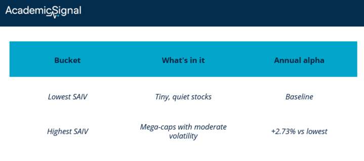
The highest SAIV bucket, which contains 79% of total market cap, earns 2.73% more annual alpha than the lowest. The statistical significance is strong (t-stat of 8.83).
The bottom line
Traditional asset pricing theory assumes idiosyncratic risk is diversifiable and therefore unpriced. This assumption requires the market portfolio to be well-diversified.
But the market portfolio today is highly concentrated. Mega-cap idiosyncratic risk doesn't diversify away – it affects aggregate wealth. Investors demand compensation for bearing it, and that compensation shows up as alpha that factor models miss.
2. Your alpha estimates are probably wrong
Not So Smart Alphas (December 10, 2025) - Link to paper
TLDR
Alpha estimates for the same fund can vary by 5x depending on methodology
Alpha needs to take into account market beta and the risk-free rate
Low R² regressions mechanically convert positive returns into "alpha"
What the author did
Lhabitant took two hedge funds with 295 months of returns and calculated their alpha twelve different ways: simple return differences, CAPM regressions, multi-factor models, and market-timing specifications.
The two funds represent opposite ends of the hedge fund spectrum.
Fund 1 is a $31 billion market-neutral multi-strategy fund (12.7% annual return, 5.3% volatility, 0.05 beta).
Fund 2 is a pure trend-following CTA (7.7% annual return, 13.2% volatility, near-zero equity beta).
Both have low correlations to traditional benchmarks; exactly the kind of funds where alpha estimation gets tricky.
The results
For the market-neutral fund, monthly alpha estimates ranged from 0.19% to 0.98% depending on method (a 5x difference). Annualized, that's the difference between 2.3% and 11.8% alpha.
For the trend-follower, estimates ranged from -0.49% to +0.69% per month. Same fund, same data, but depending on methodology, the manager is either destroying value or displaying meaningful skill.
Ways alpha estimates go wrong
1. Ignoring risk entirely. The simplest approach – subtracting benchmark returns from fund returns – assumes equal risk. A fund with beta of 1.5 will show phantom "alpha" in bull markets simply because it took more market exposure. For a market-neutral fund with 0.05 beta, almost the entire market return gets misattributed.
The naive approach: Just subtract the benchmark return from the fund return. If the fund returned 5% and the S&P 500 returned 10%, naive alpha = -5%.
The problem: This assumes the fund should have matched the market. But a fund with 0.05 beta barely moves with the market at all; it's designed to be uncorrelated.
What you'd actually expect: If the market returns 10% and your beta is 0.05, you'd only expect 0.5% of your return to come from market exposure (10% × 0.05 = 0.5%). The rest of your return is independent of the market.
A concrete example:
Say the market-neutral fund returns 1% in a month when the S&P 500 returns 8%.
Naive alpha: 1% − 8% = −7% (looks like the manager destroyed value)
Correct alpha: 1% − (0.05 × 8%) = 1% − 0.4% = +0.6% (the manager actually generated positive skill-based returns)
The naive calculation penalizes the fund for not capturing market upside it was never trying to capture.
The formula from the paper:
Naive Alpha = True Alpha + (1 − Beta) × Market Return
2. Using total returns instead of excess returns. Skipping the risk-free rate adjustment inflates alpha by (1 – Beta) × Risk-Free Rate. For a market-neutral fund with near-zero beta, almost the entire risk-free rate becomes phantom alpha. In Lhabitant's data, this pushed alpha from 0.84% to 0.98% monthly, a 17% overstatement.
The correct approach uses excess returns
You should subtract the risk-free rate from both the fund return and the market return before running the regression:
(Fund Return − Risk-Free Rate) = Alpha + Beta × (Market Return − Risk-Free Rate)
This measures how much the fund returned above the risk-free rate, relative to how much the market returned above the risk-free rate.
The shortcut some people take
Some practitioners skip this step and just regress raw total returns:
Fund Return = Alpha* + Beta × Market Return
The beta estimate comes out the same either way. But the alpha doesn't.
The math behind the bias
If you work through the algebra, the relationship between the two alpha estimates is:
Alpha* (incorrect) = Alpha (correct) + (1 − Beta) × Risk-Free Rate
A concrete example
Say the risk-free rate is 5% annually (about 0.4% monthly), and you have a market-neutral fund with beta of 0.05.
(1 − Beta) = (1 − 0.05) = 0.95
Phantom alpha added = 0.95 × 0.4% = 0.38% per month
That's 4.6% annually in fake alpha, just from skipping a simple adjustment.
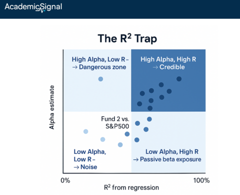
3. The R² trap. When R² is low, regressions mechanically dump positive returns into alpha. If factor returns explain nothing (low R²), the equation simplifies to: Fund Return ≈ Alpha. The fund's average return becomes the alpha estimate – not because you've identified skill, but because you've failed to identify return drivers. For the trend-follower versus the S&P 500, R² was literally 0.00%. Practical rule: if R² is below 10%, treat alpha with extreme skepticism.
The bottom line
Before concluding a manager has skill:
Run multiple models. If alpha varies wildly across specifications, you have a model problem, not an answer.
Check R². Below 10-15% explanatory power means your "alpha" is mostly unexplained returns, not demonstrated skill.
Look for omitted factors. Size, value, momentum, volatility, alternative risk premia – if the manager has exposure, it needs to be in your model.
Use appropriate benchmarks. A trend-follower compared to the S&P 500 will always show "alpha" because the benchmark explains nothing.
Respect confidence intervals. Wide intervals mean uncertainty. Don't over-interpret point estimates.
Alpha – the central metric in active management evaluation – is far less reliable than the industry pretends. We often still can't distinguish skill from noise, factor exposure, or model misspecification.
3. Research-grounded Investor Q&A: “Does unusual options activity (put-call ratio + volume spikes) predict post-earnings announcement drift direction?”
Post-2009 predictability appears driven by limits to arbitrage and macro information flow – not private information about individual firms.
What used to work: Pan and Poteshman (2003 working paper) documented that stocks with low put-call ratios (call-heavy) outperformed those with high ratios by 40 basis points per day and over 1% per week. Critically, this predictability stemmed from non-public order flow data – specifically, purchases that opened new positions – rather than publicly observable volume.
When you see "options volume" on your Bloomberg terminal or brokerage platform, you're seeing total volume. That number is noisy because it mixes together four types of trades:
Buy to open: Someone initiating a new long position (bullish if calls, bearish if puts)
Buy to close: Someone covering a previous short position
Sell to open: Someone initiating a new short position
Sell to close: Someone exiting a previous long position
Pan and Poteshman had access to a proprietary CBOE dataset that broke volume into these four categories. They found that only the "buy to open" volume predicted returns. The other three categories added noise.
The signal died in 2009. Bondarenko and Muravyev (2022 working paper) documented that put-call ratio predictability "suddenly and permanently ceased" after Raj Rajaratnam's arrest in October 2009.
The signal existed because informed traders – including those with illegal information – were trading options. When enforcement intensified, the edge vanished.
Goncalves-Pinto and Sala (2025) go further: when properly benchmarked against synthetic returns, option volume predictability is "statistically weak, economically negligible, or reverses sign."
What still works (with caveats):
Weinbaum, Fodor, Muravyev, and Cremers (2022) find option purchases predict returns on news days and ahead of unscheduled events but crucially, NOT before scheduled announcements like earnings. The original "trade options before earnings" thesis doesn't hold.
At the aggregate level, Han and Li (2023) show Implied Volatility (“IV”) spreads predict market returns out to six months, with predictability concentrating around macro news.
Disclaimer
This publication is for informational and educational purposes only. It is not investment, legal, tax, or accounting advice, and it is not an offer to buy or sell any security. Investing involves risk, including loss of principal. Past performance does not guarantee future results. Data and opinions are based on sources believed to be reliable, but accuracy and completeness are not guaranteed. You are responsible for your own investment decisions. If you need advice for your situation, consult a qualified professional.