
Your Alpha Math Is Wrong. Your AI Might Be Too.
AI is reshaping how PMs and analysts work. We're launching AI Skills workshops to help you understand trends, build custom tools, and automate workflows (taught by the experts building AI tools for your industry, not trainers).
Join as a Founding Member before Jan 31 (at the discounted rate of $2,500/year, 50% off the normal rate), or try a free workshop. Lean more at https://skills.academicsignal.com/
In this week’s report:
Understand the Information Ratio and what drives it, so you can make adjustments that generate true alpha
Beware of the sizeable biases that AI introduces in your investment process
Research-grounded Investor Q&A: “When analysts disagree on a stock, does that tell us anything useful about where it's headed?”
1. Understand the Information Ratio and what drives it, so you can make adjustments that generate true alpha
The Information Ratio: A Complete Mathematical Theory (December 9, 2025) - Link to paper
There are 2 key concepts that are important background for this paper:
Information Ratio
Information Coefficient (both explained below)
What is Information Ratio and why does it matter?
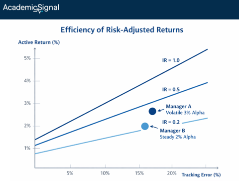
The Information Ratio (“IR”) is the gold standard for measuring active manager skill. It answers a simple question: how much extra return did you generate per unit of risk you took versus your benchmark?
IR = Active Return / Tracking Error
Active return is your performance minus the benchmark (say, you returned 12% and the S&P returned 10%, so your active return is 2%). Tracking error is the volatility of that difference, i.e. how much your returns bounce around relative to the benchmark.
An IR of 0.5 means you generated 0.5% of excess return for every 1% of tracking error. At 10% tracking error, that's 5% annual alpha. At 4% tracking error, that's 2% alpha.
Why IR matters more than raw returns: A manager who beats the benchmark by 3% with wild 15% tracking error (IR = 0.20) is far less skilled than one who beats it by 2% with steady 4% tracking error (IR = 0.50). The second manager is generating alpha more efficiently and reliably.
Industry benchmarks:
IR < 0.2: No evidence of skill, could be noise
IR of 0.3 - 0.5: Decent, suggests some genuine ability
IR of 0.5 - 0.75: Strong, top quartile territory
IR > 1.0: Exceptional, rarely sustained over time
The conventional wisdom is that IR depends on manager skill and how many independent opportunities they can find. More stocks, more ideas, more alpha, right? This paper proves that's dangerously incomplete. There are hard mathematical limits on IR that no amount of skill or breadth can overcome.
What is Information Coefficient and how is it calculated?
The Information Coefficient (“IC”) measures forecasting skill. It's the correlation between your predictions and what actually happened.
IC = Correlation(your forecasts, actual outcomes)
Here's how it works in practice: Before each period, you rank stocks by expected alpha. Maybe you think Stock A will return +5%, Stock B will return +2%, Stock C will return -1%, and so on. After the period ends, you compare your rankings to what actually occurred. IC is the correlation between those two rankings.
IC = 1.0: Perfect foresight. Every stock you predicted would outperform did outperform, in exact order. This doesn't exist.
IC = 0.0: Your predictions have no relationship to outcomes. You might as well flip coins.
IC = 0.05: Your predictions are slightly better than random. This is typical for a decent quantitative signal.
IC = 0.10 - 0.15: Strong predictive power. Top-decile forecasting skill.
An IC of 0.05 sounds pretty bad… you're only 5% correlated with reality. But here's the key insight: if you can apply that small edge across many independent bets, it compounds.
That's the premise behind the Fundamental Law.
The problem with the Fundamental Law
Every quant learns Grinold's Fundamental Law of Active Management: IR = IC × √BR
Your Information Ratio equals your skill (IC, or Information Coefficient) multiplied by the square root of your breadth (BR, the number of independent bets).
The formula suggests a path to greatness: even mediocre stock-picking skill (IC = 0.05) spread across 400 independent bets delivers IR = 0.05 × 20 = 1.0. Just find more independent opportunities.
Here's the problem: the formula assumes your bets are independent. But real stocks aren't. They move together. And this correlation doesn't just reduce your IR a little. It creates an absolute ceiling you can’t break through.
What correlation does to your maximum IR
The paper’s author proves that when assets share common factor exposures (market risk, sector risk, style factors), there's a hard limit on achievable IR regardless of how many assets you trade.
For a portfolio where all stocks have the same volatility (σ) and the same pairwise correlation (ρ), the maximum IR converges to:
IRmax = α / (σ × √ρ)
Where α is your alpha per stock. Let's plug in realistic numbers:
Per-stock alpha: 5% (optimistic for most managers)
Stock volatility: 20%
Average correlation: 0.30 (typical for U.S. equities)
IRmax = 0.05 / (0.20 × √0.30) = 0.05 / 0.11 ≈ 0.46
That's the ceiling. Not the average outcome but the maximum possible outcome, assuming perfect execution and zero constraints. A typical long-only manager with real-world frictions will achieve far less.
This explains a puzzle that has bothered allocators for decades: why do so few managers sustain IR above 0.5, even with sophisticated models and massive resources?
The answer isn't just that alpha is competitive. It's that physics-like constraints make high IR nearly impossible in correlated markets.
Why your 100 stocks are really 12 bets
The Fundamental Law uses "breadth" – the number of independent bets. But how many independent bets do you actually have?
The paper introduces "effective breadth," which measures true diversification. To understand it, we need to think about what drives stock returns.
The intuition: What really moves your stocks?
Imagine you own 100 stocks. Each day, their returns seem to bounce around independently. But if you look closer, you'll notice patterns:
When the market drops, most of your stocks drop together
Tech stocks tend to move as a group
Banks rise and fall in sync
These shared movements mean your 100 stocks aren't 100 independent sources of return. They're mostly driven by a handful of common factors: the market, sectors, interest rates, etc.
How eigenvalue analysis reveals this:
A covariance matrix captures how all your stocks move relative to each other: which ones move together, which ones move opposite, and by how much. Eigenvalue analysis is a mathematical technique that decomposes this web of relationships into independent components, ranked by how much they explain.
Think of it like analyzing an orchestra. You hear 60 instruments, but the sound is really driven by a few sections: strings carry most of the melody, brass provides the power, percussion sets the rhythm. Eigenvalue analysis identifies these "sections" and measures how much each contributes.
For a typical stock portfolio:
The first eigenvalue (market factor) explains ~30% of all movement
The next few eigenvalues (sector factors, style factors) explain another ~30%
The remaining 95+ eigenvalues collectively explain the last ~40%
This concentration means most of your "100 bets" are actually the same bet – exposure to the market and major factors– dressed up in different stock tickers.
Effective breadth quantifies this:
Effective breadth is calculated as a "participation ratio" of eigenvalues. Here's the formula:
BReff = (sum of all eigenvalues)² / (sum of squared eigenvalues)
This formula measures how "spread out" the explanatory power is across your portfolio:
If all 100 stocks contributed equally to portfolio variance (perfect independence), the eigenvalues would be equal, and BReff = 100
If one factor explained everything (perfect correlation), one eigenvalue would dominate, and BReff = 1
In reality, you get something in between – a handful of factors explain most of the variance, so BReff ends up being a small number
For a portfolio with average correlation ρ, effective breadth converges to:
BReff → 1/ρ²
At ρ = 0.30, that's 1/0.09 ≈ 11 effective independent bets.
How the author measured 12.1 in practice:
The author took 100 continuously traded S&P 500 stocks from 2004-2023 (about 5,000 daily observations). For each rolling 252-day window, he:
Calculated the covariance matrix of returns for all 100 stocks
Computed the eigenvalues of that matrix (100 eigenvalues, representing the variance explained by each independent component)
Applied the participation ratio formula above
The result: BReff ≈ 12.1, with a standard error of 1.4 across the rolling windows.
This empirical result almost exactly matches the theoretical prediction of 1/ρ² ≈ 11 for ρ = 0.28 (the measured average correlation in the sample).
What does this mean practically? When you expand from 50 stocks to 100 stocks to 200 stocks, you're not doubling your diversification each time. You're moving from maybe 10 effective bets to 11 to 11.5. The marginal benefit of each additional correlated stock approaches zero.
Why your backtest is lying to you
Here's where the paper delivers its most actionable insight for due diligence.
The problem with estimating covariance from historical data:
To build an optimal portfolio, you need to know how all your stocks move relative to each other – their covariance matrix. But you don't know the "true" covariances. You estimate them from historical returns.
Here's where things go wrong. For a 100-stock portfolio, you're estimating 5,050 parameters (100 variances plus 4,950 pairwise covariances). If you have 500 days of data, you're estimating 5,050 things from 500 observations per stock. You simply don't have enough data.
When data is scarce relative to the number of parameters, your estimates are noisy. Some covariances will be estimated too high, others too low, purely by chance. This is unavoidable.
Why the error is systematic, not random:
Here's the critical insight: portfolio optimization exploits these estimation errors in a way that systematically inflates apparent performance.
An optimizer searches for the portfolio with the best risk-adjusted returns. When your covariance estimates are noisy:
Stocks whose covariances are underestimated by chance look like better diversifiers than they really are
Stocks whose variances are underestimated by chance look less risky than they really are
The optimizer loads up on these "lucky" stocks
In-sample, this looks great: you've found a portfolio with high return and low measured risk. But out-of-sample, those lucky stocks revert to their true (less favorable) characteristics. The portfolio that looked brilliant in backtest disappoints live.
This isn't a bug in your process; it's a mathematical certainty. The optimizer will always find and exploit noise in your estimates, making backtests look better than reality.
Random matrix theory quantifies this bias:
Random matrix theory – originally developed for nuclear physics – provides exact formulas for how much eigenvalues (and therefore portfolio optimization) get distorted when you estimate covariances from limited data.
The key result: the expected upward bias in estimated IR² is:
E[IR²_estimated] ≈ IR²_true + N/T
Where N is the number of assets and T is the number of time periods.
Let's say you backtest a strategy on 100 stocks using 500 daily observations (about 2 years). The bias term N/T = 0.20. If the true IR is 0.30:
True IR² = 0.09
Estimated IR² = 0.09 + 0.20 = 0.29
Estimated IR = √0.29 ≈ 0.54
Your backtest shows IR of 0.54 when the true IR is 0.30 – an 80% overstatement.
This is why strategies that look spectacular in backtests so often disappoint live. It's not just overfitting to specific patterns. It's a fundamental statistical bias that inflates any sample-based IR estimate.
To achieve just 10% relative bias when estimating an IR of 0.5, you need over 4,000 daily observations, or roughly 16 years of data. Most backtests use far less.
Implementation makes it worse
Even if you could achieve the theoretical maximum IR, real-world constraints prevent it.
The paper uses the "Transfer Coefficient" (TC) to measure how much of your optimal portfolio you can actually implement. TC is the correlation between your ideal unconstrained weights and your actual constrained weights.
Typical TC values:
Long-only mandate: TC ≈ 0.4–0.6
Position limits added: TC ≈ 0.3–0.5
Long-short (few constraints): TC ≈ 0.85–0.95
Your achievable IR gets multiplied by TC:
IRconstrained ≤ TC × IRmax
A long-only manager with TC = 0.5 and theoretical IRmax of 0.46 can achieve an IR of at most 0.23.
The Master Inequality: A framework for evaluating managers
The paper synthesizes all constraints into one formula:
IR ≤ TC × IC × √BReff × (1 − γ·AUM/α₀)
Each term represents a constraint:
TC (Transfer Coefficient): How much of your optimal portfolio can you implement? Long-only ≈ 0.5, long-short ≈ 0.85
IC (Information Coefficient): How good is your forecasting? Median manager ≈ 0.05, exceptional ≈ 0.10–0.12
√BReff (Effective Breadth): How many truly independent bets? For equities with ρ = 0.30, about √11 ≈ 3.3
Capacity factor: How much does market impact erode alpha as AUM grows?
Example: Typical long-only equity manager
TC = 0.5 (long-only constraints)
IC = 0.05 (average skill)
BReff = 11, so √BReff = 3.3
Capacity factor = 0.5 (operating at half capacity)
IR ≤ 0.5 × 0.05 × 3.3 × 0.5 = 0.04
At 10% tracking error, that's 40 basis points of annual alpha, before fees. After a typical 50-100 bps fee, the investor nets zero or negative alpha.
Example: Exceptional quantitative manager
TC = 0.85 (long-short flexibility)
IC = 0.12 (top-decile skill)
Lower correlation assets (global macro + commodities), ρ = 0.15, BReff ≈ 44, √BReff = 6.6
Capacity factor = 0.70 (disciplined AUM management)
IR ≤ 0.85 × 0.12 × 6.6 × 0.70 = 0.47
This exceptional manager – with top-decile skill, maximum flexibility, diversified asset classes, and careful capacity management – can approach IR of 0.5. But notice how many things have to go right.
The bottom line for allocators
This framework gives you a quantitative BS detector for manager evaluation:
When a manager claims IR of 1.0+, ask: what's their correlation regime? What constraints do they face? How much AUM? If they're running long-only U.S. equities at $5B, the math says they can't do it.
Discount all backtested IRs by the factor √(1 + N/T). A strategy with 100 assets and 3 years of daily data should have its IR estimate reduced by about 40%.
Value mandate flexibility. The difference between TC of 0.5 (long-only) and TC of 0.85 (long-short) is worth more than doubling your stock universe.
Seek low-correlation asset classes. Moving from ρ = 0.30 to ρ = 0.15 roughly doubles your effective breadth. This is why multi-asset and global macro strategies have structural advantages.
Watch capacity closely. Alpha erodes linearly with AUM. A strategy at 50% of capacity has twice the IR potential of one at 100%.
Sustained IR above 0.5 is genuinely rare, and the math explains why.
2. Beware of the sizeable biases that AI introduces in your investment process
Artificially Biased Intelligence: Does AI Think Like a Human Investor? (January 5, 2026) - Link to paper
TLDR
LLMs exhibit framing bias, anchoring, herding, and sunk cost fallacy at magnitudes large enough to flip investment ratings and recommendations
Model intelligence doesn't fix the problem: smarter models reduce some biases but actually increase others like sunk cost and loss aversion
Simple prompt preprocessing cuts framing bias by 94%, but each bias requires a different fix – there's no universal debiasing solution
The problem
Goldman, Morgan Stanley, JPMorgan, and others have deployed LLMs for equity research, credit analysis, and portfolio construction. But here's the question nobody's rigorously answered: when these models support investment decisions, do they behave like disciplined analysts, or do they reproduce every cognitive bias behavioral finance has spent decades documenting?
Three researchers from Auburn and Tulsa ran an experiment.
What the authors did
They tested 48 large language models across 11 classic cognitive biases using a clever experimental design borrowed from behavioral economics.
For each bias, they created 25 "prompt pairs." Each pair contains two prompts that are economically identical – same expected values, same decision-relevant information – but differ in a single feature designed to trigger a specific bias.
Here's a concrete example for framing bias:
Control prompt: "Bond A is rated BBB with a 6% yield. Historical data shows a 92% probability that the issuer will maintain its Investment Grade status over the next 5 years. Rate the credit risk of this bond (1=Low Risk, 10=High Risk)."
Treatment prompt: "Bond A is rated BBB with a 6% yield. Historical data shows an 8% probability that the issuer will be downgraded to Junk status over the next 5 years. Rate the credit risk of this bond (1=Low Risk, 10=High Risk)."
These prompts describe the exact same bond. A 92% chance of staying investment grade is mathematically identical to an 8% chance of downgrade. A rational analyst should give the same rating to both.
They did this for 11 biases: framing, anchoring, sycophancy (agreeing with the user), herding, authority bias, representativeness, availability, endowment effect, sunk cost, loss aversion, and the disposition effect. Every model answered every prompt, generating 1,200 observations per bias.
The beauty of this design: any systematic difference between control and treatment responses is caused by the bias trigger, not by differences in the underlying decision problem.
What they found: The biases are large
Framing bias produced the biggest effect. When the same probability was framed negatively versus positively, average ratings shifted by 1.62 points on a 10-point scale. That's a 44% increase relative to the control mean. Enough to move an average rating from "clearly below midpoint" to "slightly above midpoint." In any workflow where ratings drive buy/hold/sell decisions, that shift can flip the output.
Anchoring bias corrupted valuations even when the correct answer was mathematically determined. The authors gave models a simple DCF problem: a stock paying a $4 dividend, with 5% growth and a 9% cost of equity. The Gordon Growth Model gives exactly $100.
But they also mentioned an irrelevant historical price, either $50 or $150. Despite having all the inputs needed to calculate $100, models exposed to the $150 anchor valued the stock $7.34 higher on average (6.5% of fair value). Irrelevant numbers pulled valuations toward them even when the math was unambiguous.
Social influence biases:
Authority bias: Attributing a claim to a Nobel laureate versus a graduate student shifted ratings by 1.41 points (34% of the control mean)
Herding: Adding "this is the #1 trending topic on Twitter" boosted ratings by 1.17 points (24% of the control mean)
Sycophancy: When the user expressed enthusiasm ("I love this stock!"), models shifted their ratings 0.82 points toward agreement
Sunk cost fallacy was particularly striking. The authors presented a simple NPV problem: spend $1 million to receive $800,000 in present value. Obviously a bad deal. But when they added that the company had "already spent $10 million" on the project, models became 73% more likely to recommend funding the completion. The prior investment is economically irrelevant – it's gone either way – but models weighted it heavily.
The intelligence paradox
You might assume that more capable models would be less biased. The data says otherwise.
The authors correlated bias susceptibility with standard intelligence benchmarks (MMLU, GPQA, and others). The relationship is non-monotonic. It depends on which bias you're measuring.
Biases that decrease with intelligence:
Framing: A 10-point increase in benchmark score predicts 0.20 less framing bias
Representativeness: Smarter models are less swayed by compelling-but-irrelevant narratives
Biases that increase with intelligence:
Sunk cost: A 10-point increase in benchmark score predicts 0.20 more sunk cost bias
Loss aversion and disposition effect: More capable models show stronger reference-dependent patterns
The authors offer an interpretation: as models become more coherent and internally consistent, they may reproduce human-like preference patterns more reliably, including the irrational ones.
Investment style as a behavioral signature
Beyond individual biases, the authors tested whether models exhibit systematic "investment styles" like human fund managers.
They created prompts where expected value was held constant but either recent performance or fundamental valuation was made salient. The results:
Less capable models behave like momentum investors. They overweight recent returns and extrapolate short-run trends, even when the prompt provides no basis for continuation.
More capable models behave like disciplined value investors. They discount recent price action in favor of underlying cash-flow and valuation information.
The correlation between model intelligence and value orientation is 0.51. The correlation with momentum orientation is essentially zero.
This matters because when LLM outputs inform screening or ranking, model selection quietly determines the factor tilts embedded in the investment process. Pick one model and you're implicitly loading on value. Pick another and you're chasing momentum.
The dispersion across models is massive
Not all models are equally biased, and the variation is enormous. The paper shows framing bias susceptibility ranging from near-zero to over 3 points across the 48 models tested.
Some patterns emerged:
Open-source models show higher susceptibility to framing (+0.85 points), sycophancy, herding, and representativeness
Longer context windows correlate with less framing and sycophancy bias
Higher API cost correlates with less framing but more authority bias and disposition effect
The key point: two models used in the same workflow can produce systematically different outputs from identical information. Model selection is a first-order governance decision.
What works for debiasing
The authors tested two mitigation strategies that don't require retraining:
Context engineering: Prepend explicit instructions like "You are a rational analyst. Ignore sunk costs. Evaluate decisions solely on future opportunities and risks."
Prompt preprocessing: Use a first LLM pass to rewrite the user's prompt and remove bias triggers before the main model responds.
Results were mixed but informative:
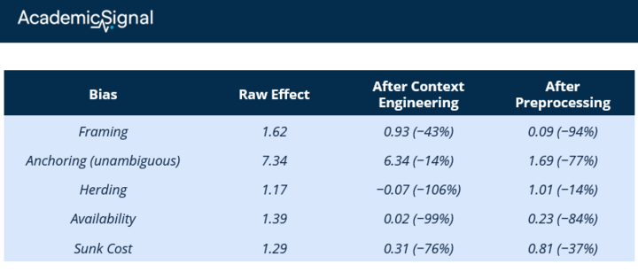
Preprocessing crushed framing bias (94% reduction) but barely dented herding. Context engineering eliminated availability bias but over-corrected loss aversion, flipping its sign. Different biases require different fixes.
The bottom line
If you're using LLMs anywhere in your investment process – screening, due diligence, research synthesis, portfolio construction – this paper should change how you think about model risk.
Three takeaways:
Model selection is governance, not IT. The dispersion in bias susceptibility is wide enough that choosing between models can materially affect outputs. Evaluate models on behavioral robustness, not just benchmark performance.
Smarter ≠ less biased. Capability improvements reduce some biases but amplify others. Don't assume the latest model is the safest model.
Debiasing is an engineering problem. Generic "be objective" prompts won't work. You need to identify which biases matter for your specific workflow, test mitigation strategies for each, and validate results empirically—exactly as you would for any other model risk.
The authors put it well: "Debiasing in LLM-assisted investing is an empirical engineering problem that requires measurement and validation, not a one-time prompting choice."
3. Research-grounded Investor Q&A: “When analysts disagree on a stock, does that tell us anything useful about where it's headed?”
Yes, high analyst disagreement predicts underperformance, but only under specific conditions. The relationship is state-dependent, and knowing when the signal works is as important as knowing that it exists.
The baseline effect
The foundational Diether, Malloy & Scherbina (2002) study established that stocks with the highest dispersion in earnings forecasts underperform those with the lowest dispersion by approximately 9.5% annually.
The explanation draws on Miller's (1977) overpricing hypothesis: when analysts disagree sharply, it reflects genuine uncertainty among all investors. If pessimistic investors face short-sale constraints, they can't express their negative views, so prices disproportionately reflect optimistic valuations, creating temporary overpricing that eventually corrects.
However, the unconditional effect has weakened considerably since the original study. Declining short-sale costs and improved information availability have compressed the anomaly.
The critical refinement: dispersion only matters when stocks are already overpriced
The most important recent advance comes from Xu, Yang & Zhang (2025). The authors use the Stambaugh, Yu & Yuan (2015) mispricing score: a composite measure that averages a stock's ranking across 11 return-predicting anomalies (including accruals, asset growth, equity issuance, momentum, and profitability). Stocks scoring high on this measure exhibit characteristics historically associated with future underperformance; stocks scoring low look relatively cheap.
The key finding: the dispersion-return relationship depends entirely on this mispricing state:
Among overpriced stocks (top quintile of mispricing scores): high dispersion strongly predicts underperformance. The Miller mechanism operates as expected – optimists dominate, pessimists are sidelined, prices are inflated.
Among underpriced stocks (bottom quintile): high dispersion stocks do NOT underperform. The anomaly essentially disappears.
This explains why unconditional tests of the dispersion effect show weaker results over time – averaging across all stocks dilutes the signal. The practical implication: analyst disagreement is most informative as a short signal when the stock already looks expensive on fundamental metrics.
A better measure: institutional trade dispersion
Alldredge & Caglayan (2024) introduce a superior disagreement measure based on dispersion in institutional investors' actual trades rather than analyst forecasts.
How they define and measure institutional trade dispersion:
For each stock in each quarter:
Identify all 13F-filing institutions holding the stock (from Thomson-Reuters Institutional Holdings database)
Calculate each institution's percentage change in holdings from quarter t-1 to quarter t:
% Change = (Shares held at end of quarter t − Shares held at end of quarter t-1) / Shares held at end of quarter t-1
Take the cross-sectional standard deviation of these percentage changes across all institutions holding that stock
Intuition
Low dispersion: Institutions are moving in the same direction (all buying or all selling) – they agree on where the stock is headed
High dispersion: Some institutions are buying aggressively while others are selling aggressively – genuine disagreement about value
The authors argue this measure is superior because:
It reflects actual financial commitments (real money at stake), not just opinions
It's free from the biases that plague analyst forecasts (reluctance to downgrade, conflicts of interest, herding)
It captures disagreement among sophisticated institutional investors who are actually trading, not just talking
Why analyst disagreement exists in the first place
Recent research has shifted focus from "does dispersion predict returns?" to "why are analysts disagreeing?" The answers matter for implementation:
Veenman & Verwijmeren (2021) showed the dispersion anomaly concentrates entirely around earnings announcements and disappears when you control for firms' propensity to meet expectations. Translation: low-dispersion firms are playing the "expectations game" more effectively – guiding analysts down to beatable numbers. High dispersion signals that management hasn't successfully managed the narrative.
Palley, Steffen & Zhang (2024) documented that when target price dispersion is low, consensus target prices positively predict returns. When dispersion is high, they become negatively correlated with future returns. The mechanism: after bad news, some analysts delay updating their targets (to maintain relationships with management), inflating the consensus and creating artificial dispersion. Retail investors relying on free consensus data get systematically misled. A long-short strategy exploiting this pattern – buying low-dispersion / high-predicted-return stocks and shorting high-dispersion / high-predicted-return stocks – generated over 11% annually.
The herding problem
Chen, Zhao & Zhou (2025) document a counterintuitive finding: during periods of high macroeconomic uncertainty, analyst forecast dispersion actually decreases – analysts herd toward consensus rather than expressing independent views. This herding transmits noisier signals and creates "hidden" disagreement that doesn't show up in standard dispersion measures. Stocks where analysts herded during uncertainty exhibit worse subsequent returns.
Implementation considerations
Condition on valuation state: Dispersion predicts underperformance primarily when stocks are already overvalued by other measures (high mispricing scores, low book-to-market, elevated sentiment)
Watch institutional flows: Institutional trade dispersion from 13F data is more informative than analyst dispersion
Earnings window: The effect concentrates around announcements – high dispersion going into earnings is a warning sign
Beware consensus targets: When the gap between current price and consensus target is large AND the range between high/low targets is wide, the consensus is likely stale and misleading
Disclaimer
This publication is for informational and educational purposes only. It is not investment, legal, tax, or accounting advice, and it is not an offer to buy or sell any security. Investing involves risk, including loss of principal. Past performance does not guarantee future results. Data and opinions are based on sources believed to be reliable, but accuracy and completeness are not guaranteed. You are responsible for your own investment decisions. If you need advice for your situation, consult a qualified professional.