
Machine Learning Just Found a Better Way to Build Portfolios
We're launching AI Skills: Learn AI by the Builders in your industry
It’s a series of workshops to help you understand trends, build custom tools, and automate workflows. Each taught by a CTO / Head of AI building in the investment industry.
Reply “SKILLS” to join as a Founding Member (the first 100 get a 50% discount for life) or lean more at https://skills.academicsignal.com/
In this week’s report:
You can boost returns without increasing volatility by integrating portfolio optimization into your ML training – rather than first predicting returns, and then optimizing allocation
IRR without a time dimension can be misleading – this “endurance” measure fixes it
Research-grounded Investor Q&A: “Should a publicly-traded company with substantial foreign operations hedge its currency risk, or leave it to investors?”
1. You can boost returns without increasing volatility by integrating portfolio optimization into your ML training – rather than first predicting returns, and then optimizing allocation
Machine Learning Meets Markowitz (January 1, 2026) - Link to paper
The prediction-optimization disconnect
Most quantitative strategies follow a two-stage process that dates back decades.
In stage one, you train a model (whether linear regression, random forest, or neural network) to predict returns across your entire stock universe. The model’s objective is to minimize mean-squared error (MSE): it looks at its predicted return versus the actual return for every stock-day observation, squares the difference (so big misses count more than small ones), and averages across millions of data points. The algorithm then tweaks its parameters to shrink that average squared error as much as possible.
This sounds sensible, but it creates a subtle problem. MSE treats every prediction error as equally important. A 1% forecast miss on Apple counts the same as a 1% miss on a microcap you'll never trade. The model has no idea which stocks will end up in your portfolio, so it's trying to be accurate everywhere. Everyone using that model gets identical expected return estimates.
In stage two, you hand those predictions to an optimizer. The classic approach – dating back to Harry Markowitz in 1952 – frames portfolio construction as a tradeoff between expected return and risk. The optimizer maximizes your portfolio's expected return (using those ML forecasts) minus a penalty for portfolio variance (using a covariance matrix estimated from historical returns). How much you penalize variance depends on your risk aversion parameter: crank it up and you get a diversified, lower-volatility portfolio; dial it down and you concentrate in your highest-conviction names.
On top of this return-versus-risk objective, you layer constraints: long-only (no shorting), maximum position sizes, sector limits, turnover caps. The optimizer takes your forecasts, covariance matrix, risk aversion, and constraints as fixed inputs, then solves for the portfolio weights that maximize your objective. It has no say in how the predictions were generated; it just takes them as given.
This raises a couple of problems:
Problem 1: The returns-forecasting model doesn't know your risk preferences. A risk-averse pension fund and an aggressive hedge fund get identical return forecasts, even though they'll build completely different portfolios.
Consider a simple example: your model predicts Stock A will return 15% with high volatility, while Stock B will return 8% with low volatility. The pension fund will overweight Stock B; the hedge fund will load up on Stock A.
BUT the MSE-trained model spent equal effort getting both forecasts right. It would have been better for the pension fund if the model focused its predictive power on low-volatility names, and vice versa for the hedge fund. One-size-fits-all predictions leave alpha on the table for everyone.
Problem 2: The model doesn't see transaction costs. ML models love short-term reversal signals: stocks that dropped yesterday tend to bounce today. These signals show up as highly predictive in backtests. But capturing them requires massive portfolio churn. The authors found turnover rates around 60% per day. At realistic transaction costs of 20-30 basis points per trade, that turnover eats your entire alpha. The paper shows traditional MSE models turn unprofitable at 30 bps transaction costs, while the E2E approach stays positive. The MSE model literally cannot adapt because it never learned that turnover matters.
Wang, Gao, Harvey, Liu, and Tao argue this separation is fundamentally misaligned with how investors actually make decisions. A concentrated hedge fund needs pinpoint accuracy on its top holdings, not marginally better forecasts for stocks it will never own.
How they built it
The authors constructed an "end-to-end" (E2E) framework that embeds the portfolio optimization problem directly into the neural network training loop. Instead of minimizing mean-squared prediction error, the model learns parameters that maximize the realized utility of the resulting portfolio.
Here's the key insight: in a traditional setup, the neural network makes predictions, then a completely separate optimizer builds a portfolio from those predictions. The neural network never finds out what portfolio got built or how it performed. It's like training a chef by grading their ingredient prep without ever tasting the final dish.
E2E flips this. After the neural network makes predictions, those predictions flow into an optimizer that constructs a portfolio, and this optimization step is embedded inside the training loop. The model then sees the actual portfolio returns, and adjusts its parameters to improve those returns directly.
Crucially, this is not an iterative refinement of the two-stage approach. You don't run MSE first, see which stocks mattered, then re-run MSE on those stocks. It's a single unified training loop where the loss function is portfolio return, not prediction error. The neural network never sees an MSE objective. Its only goal is: "did the portfolio I helped build make money?"
The result: if you're building a long-only top-decile portfolio, the model learns to get the ranking right at the top, even if that means slightly worse predictions for stocks that will never make the cut. If you're penalizing turnover, the model learns to downweight signals that cause excessive trading. The training objective matches the investment objective.
What they found
For long-only portfolios, E2E delivered 42.5% annualized returns versus 38.0% for the traditional approach. The Sharpe ratio jumped from 1.86 to 2.08.
The real power shows up when you add frictions. At 20 basis points transaction cost, E2E returned 29.1% net versus 24.0% for the two-stage approach. At 30 bps, traditional models turned negative while E2E stayed positive at 23%. The mechanism: E2E dynamically down-weights high-turnover signals like short-term reversal as trading costs rise.
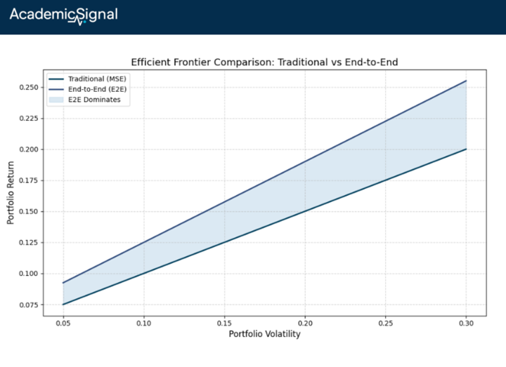
For investors with different risk appetites, the performance gap widens dramatically. Aggressive allocators earned 71% annually with E2E versus 50% with MSE. The E2E frontier consistently dominated, achieving higher returns at every risk level.
Why this matters
It's tempting to think the fix is simpler: just train your MSE model on a narrower universe. If you're a healthcare-focused fund, train only on healthcare stocks. But this misses the point. MSE on a smaller universe still treats every stock's prediction error equally. It still ignores your constraints, risk preferences, and transaction costs. You've shrunk the problem without solving it.
The E2E insight is more fundamental: change what you optimize, not just which stocks you include. By embedding portfolio construction inside the training loop, the model discovers which predictions actually move the needle for your specific strategy.
A long-only fund automatically gets a model that focuses on ranking accuracy at the top. A turnover-constrained fund gets a model that favors persistent signals. The feedback loop “predictions → portfolio → returns → gradient update” cannot be replicated by filtering your training data.
The bottom line
If you're running ML-based strategies with real-world constraints, you're likely leaving alpha on the table with the standard predict-then-optimize workflow. The E2E approach offers a systematic way to train models that respect your actual investment mandate. The gains are largest for concentrated, cost-sensitive, or constraint-heavy portfolios – exactly where most institutional capital lives.
2. IRR without a time dimension can be misleading – this “endurance” measure fixes it
Endurance of Internal Rate of Return (January 16, 2026) - Link to paper
TLDR
IRR without a time horizon is incomplete: a 30% IRR over 3 years of effective capital deployment is very different from 30% over 10 years
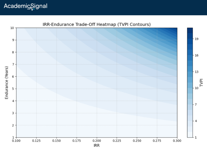
"Endurance" measures the effective time your capital actually compounds at the stated IRR: divide the natural log of TVPI (total value to paid-in capital, i.e., distributions plus remaining value divided by contributions) by the IRR
What the author did
Vishv Jeet tackled a problem every LP knows but rarely quantifies: IRR can mislead. A fund reporting 30% IRR sounds impressive, but if that rate only applies for 3 effective years rather than the fund's 15-year life, you're not getting 15 years of 30% compounding. The paper introduces a simple metric called "endurance" that makes the implicit time dimension explicit.
How to calculate “endurance”
The formula comes from solving the continuous compounding equation backwards for time.
If total contributions (TC) compound at rate r for time t, they grow to total distributions (TD):
TD = TC × e^(r × t)
Dividing both sides by TC gives TVPI = e^(r × t). Take the natural log of both sides: ln(TVPI) = r × t. Solve for time:
Endurance = ln(TVPI) / IRR
In plain terms, endurance answers: "If I invested all contributions on day one and they compounded continuously at the stated IRR, how many years would it take to reach my total distributions?" It backs out the implied time from the observed rate and multiple.
For example: a fund with 2.5x TVPI and 30% IRR has endurance of ln(2.5)/0.30 ≈ 3.1 years. The 30% return sounds great, but it only compounds for about 3 years – not the fund's full 15-year life. The rest of the time, your capital either hasn't been deployed or has already been returned.
A caveat on compounding conventions: The paper uses continuous compounding, but standard IRR uses discrete (typically annual) compounding. For a 20% rate over 5 years, discrete compounding gives 2.49x while continuous gives 2.72x (~9% difference). The continuous formula works as an approximation because ln(1 + IRR) ≈ IRR for lower rates. But at higher IRRs the gap widens: ln(1.30) = 0.26, not 0.30. For precision, the discrete version would be: Endurance = ln(TVPI) / ln(1 + IRR). Use this if you're implementing in practice with high-IRR funds.
What they showed
Using a large dataset of U.S. private capital funds across buyout, venture, real estate, and real assets, the authors found:
Funds with identical IRRs often have vastly different endurance profiles
High IRRs in venture capital frequently pair with short endurance – capital turns over quickly through early exits
Real estate and infrastructure show lower IRRs but longer endurance – money compounds patiently over more years
Two funds can deliver identical TVPI through completely different paths: one with high IRR/short endurance (fast money, quick exits), another with lower IRR/long endurance (steady compounding). The liquidity and reinvestment implications are night and day.
Why this matters for due diligence
When a GP pitches a 25% net IRR, ask: "What's the endurance?" If it's 2 years on a 10-year fund, most of your commitment sat idle or was already returned. The fund might look efficient, but your actual capital deployment was brief. Meanwhile, a 15% IRR with 8-year endurance means your money worked longer.
This directly affects portfolio construction. Short-endurance funds require faster capital recycling to maintain exposure. Long-endurance funds tie up capital but deliver steadier compounding.
How to use endurance in practice
If two funds offer the same IRR, the one with higher endurance is unambiguously better. Rearranging the formula shows that TVPI = e^(IRR × Endurance), so for a fixed IRR, higher endurance means higher total value created.
The harder question is comparing different IRRs with different endurances. A 25% IRR over 4 years of endurance and a 20% IRR over 5 years both give you roughly the same TVPI (~2.7x).
But there's a catch: short endurance means your capital comes back faster, which sounds good, but now you face reinvestment risk. Can you redeploy that capital at the same IRR? If your next best opportunity is 12%, then a fund with 20% IRR and 6-year endurance beats a fund with 25% IRR and 3-year endurance, because the first fund locks in that rate longer.
The paper doesn't give a precise "how much lower IRR tips the scales" formula, but the mental model is: endurance is like bond duration. In a falling-rate environment, you want longer duration to lock in today's rates. Same logic applies here: if you're skeptical you can reinvest at similar IRRs, favor endurance.
The bottom line
Add one line to your fund analysis: ln(TVPI)/IRR = endurance. Report IRR and endurance together. A high IRR with short endurance reflects quick turnover, not sustained compounding. For LPs managing cash flows and pacing models, endurance translates headline performance into what actually matters: how long your capital effectively works at the stated rate.
3. Research-grounded Investor Q&A: “Should a publicly-traded company with substantial foreign operations hedge its currency risk, or leave it to investors?”
Yes, and here's why the "shareholders can hedge themselves" argument collapses in the real world.
The Modigliani-Miller framework predicts that if shareholders can replicate corporate hedging through their own portfolio adjustments ("homemade leverage"), then corporate hedging adds no value. In perfect markets, this holds. But five documented market frictions make corporate-level hedging superior to shareholder-level hedging:
1. Cashflow Volatility Leads to Underinvestment (most robust finding)
The seminal Froot, Scharfstein & Stein (1993) model demonstrates that when external financing is costlier than internal funds, hedging creates value by ensuring cash availability for positive-NPV investments.
Berrospide, Purnanandam & Rajan (2010) provided causal evidence using Brazilian firms during the 1999 currency crisis: currency derivative users had valuations 6.7-7.8% higher than non-users. Critically, hedged firms' capital expenditure was completely insulated from operating cash flow variation – non-hedgers' investment was tightly constrained by internal funds.
This directly validates the Froot-Scharfstein-Stein prediction that shareholders cannot replicate this benefit because they cannot inject capital into the firm at the precise moment distressed operating conditions require it.
2. The Valuation Premium (PE multiple effect)
Allayannis & Weston (2001) documented that firms using foreign currency derivatives trade at Tobin's Q valuations 4.87-5.7% higher than non-hedgers.
However, Magee (2009) raised endogeneity concerns. After controlling for feedback effects (highly valued firms may hedge more), the direct causal effect weakens.
The more robust finding is the mechanism through which value is created: reduced earnings and cash flow volatility translates directly into higher valuation multiples.
Barnes (2002) found a significantly negative relationship between earnings volatility and market-to-book ratios, controlling for size, leverage, and growth. This relationship persists even after controlling for underlying operating cash flow volatility, meaning that accounting-driven earnings smoothing via hedging provides real economic value.
The valuation premium mechanism works as follows: investors discount volatile earnings streams more heavily because volatility (1) impairs earnings predictability, and Dichev & Tang (2009) confirm the strong inverse relationship, (2) increases perceived risk of financial distress, and (3) signals uncertain investment opportunities. Corporate hedging reduces this discount.
3. Shareholders Cannot Replicate Corporate Hedging
The "homemade hedging" critique fails for several reasons shareholders face but corporations don't:
Transaction costs: Retail investors face meaningfully higher bid-ask spreads and margin requirements in currency derivatives markets than corporate treasury operations
Information asymmetry: DeMarzo & Duffie (1991, 1995) showed that shareholders cannot observe the firm's true currency exposure with precision. Corporate hedging eliminates "noise" in earnings that would otherwise require shareholders to expend resources diagnosing
Scale economies: Meta-analyses by Arnold et al. (2014) consistently confirm that hedging exhibits economies of scale. A firm with $500M in euro-denominated revenues can hedge more efficiently than 10,000 shareholders individually hedging their fractional exposure
Timing and coordination: Shareholders cannot synchronize their hedging with the firm's operational cash flow timing or investment needs
4. Smoothed Earnings Increase Debt Capacity
Graham & Rogers (2002) found that hedging increases firm debt capacity, which generates tax shield value.
Leland (1998) showed that reduced financial distress probability from hedging allows firms to carry more leverage without increasing credit risk. This is something shareholders absolutely cannot replicate. Your personal hedging cannot affect the firm's borrowing costs or debt capacity.
5. Recent Evidence and Meta-Analysis
A comprehensive meta-analysis of the corporate hedging literature by Lievenbrück & Schmid (2014) covering 73,000+ firms confirms: the bankruptcy/financial distress hypothesis receives the strongest empirical support.
Firms hedge more when they face higher expected distress costs (proxied by leverage, liquidity constraints, and firm size).
Ahmed & Guney (2022) find that financial hedging directly reduces UK firms' cost of equity capital by lowering stock return volatility – a mechanism unavailable to shareholders hedging personally.
Practical Caveats
The hedging premium is not universal. Jin & Jorion (2006) found no significant hedging premium for oil and gas producers, likely because investors want commodity exposure when buying those stocks.
Lookman (2009) found that hedging "big" risks (core business exposures) may signal management weakness, while hedging "small" risks (peripheral exposures) signals prudence.
The implication: hedge currency risk when it's incidental to your business model, not when investors specifically bought your stock for that exposure.
Disclaimer
This publication is for informational and educational purposes only. It is not investment, legal, tax, or accounting advice, and it is not an offer to buy or sell any security. Investing involves risk, including loss of principal. Past performance does not guarantee future results. Data and opinions are based on sources believed to be reliable, but accuracy and completeness are not guaranteed. You are responsible for your own investment decisions. If you need advice for your situation, consult a qualified professional.